Mastering Logistic Regression: Step-by-Step Implementation in Python with Visualisation .

 

        Logistic Regression is one of the most fundamental yet powerful algorithms in machine learning for binary classification. In this article, we’ll dive deep into how it works — from the theory and maths to a complete implementation in Python without using any ML libraries like Scikit-learn.

Before going to dive deep , we need to understand some related terminologies , these are following :

Sigmoid Function:
A mathematical function that maps any real number input value to a value between 0 and 1 — used to convert outputs into probabilities. The given formula is to calculate Sigmoid function.

                         

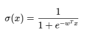
Where x = input feature vector .
w = weight vector.
w^T .x= dot product of weights and inputs.
Eg. consider Input vector x=[1,75]x = [1, 75]x=[1,75]
Weight vector w=[0.5,0.01]w = [0.5, 0.01]w=[0.5,0.01]
wTx=(0.5×1)+(0.01×75)=0.5+0.75=1.25
Now apply to Sigmoid:

           

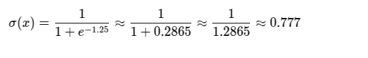
Here we get output as 0.77 for our input 75.

2. Decision Boundary :
In logistic regression, the decision boundary is the point where the model changes its prediction from one class to another (like from class 0 to class 1). It divides the feature space into two areas: one where the model predicts class 0, and the other where it predicts class 1.

In logistic regression, a threshold value is set (typically 0.5). If the predicted probability is greater than or equal to this threshold, the input is classified as class 1. If the predicted probability is smaller than the threshold, the input is classified as class 0.
According to this the above input will be classified into class 1.

3 .Cost Function and Gradient Descent:
In logistic regression, we use a cost function to measure how well the model’s predicted values align with the actual outcomes. Since logistic regression deals with binary classification, we cannot use the normal squared error (as in linear regression). Instead, we use the log loss or binary cross-entropy cost function.

Cost Function Formula:

To minimize this cost, we use Gradient Descent, an iterative optimization algorithm that adjusts the model’s parameters to reduce the cost.

Implementation for Each step in Python:

We will now implement each step of logistic regression from scratch, without using any external libraries like sklearn.

1. To calculate Sigmoid Function (For hypothesis):

def hypothesis(X,theta):
    return Sigmoid(np.dot(X,theta))

def Sigmoid(z):
    return 1/(1+np.exp(-z))

2 . classifies hypothesis based on Decision Boundary:

def predict(X,theta):
    prob=hypothesis(X,theta)
    return (prob>=0.5)

3. Updating Parameters by Gradient Descent :

def gradient_descent(X, y, theta, lr=100, epochs=1000):
    m = len(y)
    for i in range(epochs):
        h = hypothesis(X, theta)
        gradient = (1 / m) * np.dot(X.T, (h - y))
        theta -= lr * gradient
    return theta

Below is the complete implementation of Logistic Regression from scratch, combining all the steps we discussed earlier.

import numpy as np
import pandas as pd
from sklearn.model_selection import train_test_split
from sklearn.preprocessing import LabelEncoder, StandardScaler


df = pd.read_csv("Customer_Data.csv")

le = LabelEncoder()
df['Gender_encoded'] = le.fit_transform(df['Gender'])  # Male=1, Female=0

# Extract features (X) and label (y)
X = df[['Age', 'EstimatedSalary', 'Gender_encoded']].values
y = df['Purchased'].values.reshape(-1, 1)

# Normalize X
scaler = StandardScaler()
X = scaler.fit_transform(X)

X = np.hstack([np.ones((X.shape[0], 1)), X])  # Shape becomes (m, n+1)

theta = np.zeros((X.shape[1], 1))  # Shape: (n+1, 1)

def sigmoid(z):
    return 1 / (1 + np.exp(-z))


def hypothesis(X, theta):
    return sigmoid(np.dot(X, theta))


def gradient_descent(X, y, theta, lr=100, epochs=1000):
    m = len(y)
    for i in range(epochs):
        h = hypothesis(X, theta)
        gradient = (1 / m) * np.dot(X.T, (h - y))
        theta -= lr * gradient
    return theta

# Predict using threshold = 0.5
def predict(X, theta):
    probs = hypothesis(X, theta)
    return (probs >= 0.5) 

# Split data
X_train, X_test, y_train, y_test = train_test_split(X, y, test_size=0.2, random_state=42)

# Train
theta_final = gradient_descent(X_train, y_train, theta)

# Predict
y_pred = predict(X_test, theta_final)

# Accuracy
accuracy = np.mean(y_pred == y_test)
print("Final Accuracy:", accuracy.__round__(2)*100,"%")

To download the CSV file used in this implementation click Here

Evaluation of Model:

Final Accuracy: 91.0 %

The accuracy of the model is 91%, meaning approximately 91% of the predictions made by the model on the test data are correct.

The model predicts whether a customer will make a purchase based on features such as Gender, Age, and Estimated Salary. To enhance understanding and visualisation, we can utilize the Weka tool for graphical representation and analysis.

The plot matrix shows how features like Gender, Age, and Estimated Salary relate to the Purchased outcome. Generated using Weka, it highlights how logistic regression separates customers who purchased (orange) from those who didn’t (blue).
Age and Estimated Salary are strong predictors — purchasers tend to be older and earn more.
Gender has little impact, as data points are evenly spread.
The model’s decision boundary is visible through the clear separation in the scatterplots.

Advantages of Logistic Regression :

• Simple and easy to implement.
• Interpretable coefficients for understanding feature impact.
• Works well for binary classification problems.
• Efficient to train and computationally less expensive.

Disadvantages of Logistic Regression:

• Assumes linear relationship between features and the log-odds.
• Not suitable for complex relationships without feature engineering.

Applications of Logistic Regression:

• Medical diagnosis (e.g., predicting diseases like diabetes or cancer).
• Credit scoring and risk assessment in finance.
• Customer purchase prediction in marketing.
• Email spam detection.
• Customer churn prediction.
• Voting behaviour analysis.
• Fraud detection in banking and e-commerce.

Thank you for reading! If you found this article helpful, feel free to show your support by clapping (up to 50 times). Let’s connect on LinkedIn .